
Abstract
Since the advent of deep learning, solutions for machine learning problems, ranging from image classification to computer vision to natural language processing, have been revolutionized at an unprecedented rate. The data in these datasets are represented in Euclidean space. Nonetheless, there has been a surge in non-Euclidean data and graph applications in recent years, which adds complexities to current machine learning algorithms due to the independence and complicated relations between graph nodes, motivating a new line of research aiming to generalize existing deep learning methods to graph data. In this literature review, I explore five papers in this field.
Introduction
For generalizing deep learning methods to graphs, different architectures have been inspired by existing deep learning architectures such as RNNs, CNNs, and autoencoders, which have been employed on graphs.
Deep learning methods can effectively learn representations for Euclidean data, but these methods are not adequate for graph data, a relational data type, due to its inherent complexity. One primary presumption in these methods is that instances are independent of each other, which is not met in the graph domain due to the node interconnections. Additionally, graphs may have different numbers of nodes and different node degrees (irregular graphs), adding extra complexity.
Graph neural networks using recurrent structural models capture node dependencies through message passing, in which node representations are derived from neighborhood information. Since images can be considered as a special form of graph data, CNN architecture has been employed in the graph domain, leading to the development of graph convolutional neural networks, which generate node representations using convolution operations.
Preliminaries
In this section, we will introduce the mathematical formalism of Graph Neural Networks, alongside a brief introduction to primary concepts.
Formulation
Consider the graph \(G = (V, E)\), where \(V \in \{1,2,...,n\}\) is the set of nodes, and \(E \in V \times V\) is the set of edges. Let \(x_i\) be the corresponding feature vector for node \(i\), and \(e_{ij}\) be the feature vector for the edge between node \(i\) and node \(j\).
Weisfeiler-Lehman Test
The Weisfeiler-Lehman (1-WL) test [1] is a popular algorithm for checking graph isomorphism. This test is used in graph learning literature as a tool for assessing the power of graph models.
Readout(Pooling) Function
The crucial step in various learning tasks with graph neural networks is the successful combination of node features into a representation at the graph level using read-out functions. Generally, these read-out(pooling) functions are designed to be straightforward and not adaptable, ensuring that the resulting space of hypotheses remains invariant to permutations. Average, max, min pooling are common graph pooling functions.
Message Passing Framework
Consider graph \(G\), where each node has a hidden feature vector \(h^{t+1}\), derived from the last layer feature vectors \(h^t\) and messages from neighbors \(m^{t+1}\).
\begin{equation} h_v^{t+1} = U_t(h_v^t,m_v^{t+1}), :where : m_v^{t+1} = \sum_{u \in N(v|G)} M_t(h_v^t,h_u^t,e_{uv}) \end{equation} \(U_t\) and \(M_t\) represent the message and update functions, while \(N(v|G)\) denotes the set of neighbors of node \(v\). After T layers of message passing, the final representation of node \(v\) is denoted as \(h^T\).
Graph representation is then calculated using the readout function: \begin{equation} h_G = R({h_v^T | v \in G}) \end{equation} The message-passing framework iteratively aggregates node information and assigns the derived representation to the center node to capture local structural information.
1-Hop Message Passing Framework
This framework is the same as what was mentioned in section 2.4, with one slight difference: it emphasizes that the contribution of neighboring nodes should be collected from neighbors with a distance equal to 1.
Homophily Assumption
GNNs are constructed based on the homophily assumption [2], which posits that connected nodes are likely to have similar attributes, providing supplementary information beyond node features. This relational inductive bias, as indicated in [3], is considered a significant factor contributing to the superior performance of GNNs compared to traditional neural networks in numerous tasks. A homophily value nearing 1 signifies strong homophily for similarity, whereas a value approaching 0 signifies strong heterophily.
Heterophily
Despite the superior performance of GNNs, there have been some tasks with relational data where classic deep learning models such as MLP outperform GNNs due to the heterophily problem. Heterophily is widely believed to be detrimental for message-passing based GNNs [4], which occurs when homophily is no longer maintained, and connected nodes have different features.
Reviewed Papers
Nested Graph Neural Networks [5]
The Message Passing framework mentioned in section 2.4 is, at most, as powerful as the 1-WL test for distinguishing non-isomorphic graphs. This framework constructs a subtree for each node, with that node as the root. Similarly, the 1-WL test utilizes message passing to build a subtree around each node as a central node, and two graphs are classified into the same class if they have many similar subtrees. However, a rooted subtree represents only one specific substructure and is not versatile enough to represent arbitrary subgraphs, particularly those with cycles due to the inherent limitations of tree structures.
This paper proposes Nested Graph Neural Networks to overcome this inherent limitation of message passing frameworks. The main idea is to encode subgraphs for central node representation instead of encoding subtrees. Subgraphs are more informative structures for representing graph features and are not restricted to specific types of graphs. Additionally, they exploit the local structure around each node.
To represent a graph using subgraphs, NGNN uses two levels of GNN: the inner and outer levels. First, local subgraphs are extracted for each node, and then the inner GNN is applied to these subgraphs. After this stage, a pooling layer is applied to extract subgraph representation using neighboring node representations as central node representation. Eventually, by applying another pooling layer on central node representations, the graph representation for the original graph is obtained. Also, the inner GNNs are applied independently in each subgraph.
Message Passing Limitations
Because his framework iteratively encodes neighboring nodes’ information to obtain central node representations, a subtree is encoded for each node. Nonetheless, the inherent representational restriction of subtrees leads to the power of the neural network being at most as powerful as the 1-WL test. The underlying reason for this is that a subtree is a specific and restricted structure, not generalizable to all graph structures.
NGNN Framework
To obtain the final representation of each node, the corresponding subgraph should be encoded by applying the inner GNN to it. The choice of the type of inner GNN is optional, but the NGNN paper uses message-passing-based graph neural networks. First, T steps of message passing are needed to obtain the representation for the central node w from its local subgraph. The representation of node v in the subgraph of central node v is as follows:
\begin{equation} h_{v,G_w^{h^{t+1}}} = U_t(h_{v,G_w^{h^{t}}},m_{v,G_w^{h^{t+1}}}), \space where \; m_{v,G_w^{h^{t+1}}} = \sum_{u \in N(v|G_w^{h})} M_t(h_v^t,h_u^t,e_{uv}) \end{equation} \(G_w^{h}\) is the subgraph for central node \(w\). After T steps of message passing, a pooling layer is applied to obtain subgraph representations, which are used as the central node representations.
\begin{equation} h_w := h_{G_w^{h}} = R_0({h_{v,G_w^{h}}^T | v \in G_w^{h}}) \end{equation}
By employing an outer GNN, here, a pooling layer can be used, but GNNs are also applicable for this level on central nodes. All nodes have been considered as the central node once, and the representation for the original graph is obtained.
\begin{equation} h_G := R_1({h_w | w \in G}) \end{equation}
NGNN can be considered a two-level network of networks. The inner network learns each node’s representation, while the outer network is responsible for the whole graph’s representation. NGNN has changed the receptive field of each node from a subtree to a subgraph. Since the representations of each node are calculated multiple times in different subgraphs, each node can have more than one representation.
The representation power of NGNN
The representation power of NGNN surpasses message passing graph neural networks. While conventional graphs cannot be distinguished by message-passing GNNs, NGNN can effectively discriminate among these graphs. Therefore, the representation power of NGNN exceeds that of 1-WL and 2-WL tests. However, its performance compared to 3-WL tests is still not fully understood.
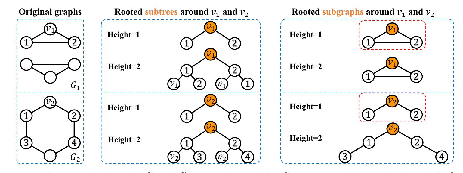
Figure 1 demonstrates the enhanced discriminative power of NGNN since it is capable of discriminating circular graphs. Lastly, NGNN is a framework that allows other GNNs to be used in a plug-and-play fashion as inner and outer GNNs.
How Powerful are K-hop Message Passing Graph Neural Networks [6]
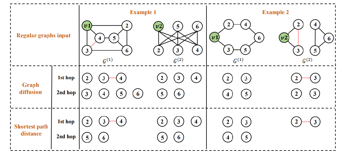
The concept of message passing between neighbors with a distance of 1 was discussed in section 2.5. The representation power of these GNNs is bounded by the 1-WL test and cannot distinguish two non-isomorphic graph structures if the 1-WL test fails. K-hop message passing is a type of message passing where the node representation is updated by aggregating information from not only the 1st hop but also all the neighbors within K hops of the node. This paper theoretically characterizes the expressive power of K-hop message passing GNNs.
1) it formally distinguishes between two different kernels of the K-hop neighbors. The first kernel is based on whether the node can be reached within k steps of the graph diffusion process, which is used in GPR-GNN [7] and MixHop [8]. The second one is based on the shortest path distance of k, which is used in GINE+ [9] and Graphormer [10].
2) This paper demonstrates that K-hop message passing surpasses the capabilities of 1-hop message passing and can effectively differentiate nearly all regular graphs.
3) Because K-hop message passing remains ineffective at distinguishing certain basic regular graphs, regardless of the chosen kernel, and its expressive capacity is limited by the 3-WL test, this serves as motivation for this paper to enhance K-hop message passing even more.
K-hop Message Passing Framework
The framework of 1-hop message passing can be straightforwardly extended to K-hop message passing, as it shares the same message and update mechanisms. The distinction lies in the ability to employ independent message and update functions for each hop. Additionally, a combination function is required to merge the outcomes from different hops into the final node representation at this layer. This paper initially distinguishes between two distinct kernels for K-hop neighbors, which have previously been interchanged and misused in prior research.
The first kernel for K-hop neighbors is known as the shortest path distance (SPD) kernel. In other words, the k-th hop neighbors of a node \(v\) in graph \(G\) consist of nodes with a shortest path distance of \(k\) from \(v\).
The second kernel for K-hop neighbors is based on graph diffusion (GD). It comprises a set of nodes that, after \(k\) hops, can diffuse messages to the node \(v\). K-hop message passing exhibits certain limitations, such as being bounded by the 3-WL test and the importance of selecting the appropriate kernel type.
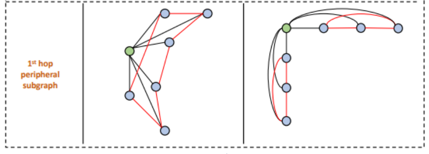
KP-GNN
This paper proposes KP-GNN to overcome k-hop messaging shortcomings. Moreover, it also utilizes k-hop message passing on peripheral subgraphs (Figure 3).
Revisiting Heterophily For Graph Neural Networks [11]
In section 2.6, we discussed the tendency of GNNs to rely on the homophily assumption [12]. However, the absence of homophily, known as heterophily, is considered a significant factor contributing to the lower performance of GNNs in certain tasks [4]. This paper takes a fresh look at homophily metrics and, additionally, explores heterophily from the perspective of post-aggregation node similarity.
It introduces new homophily metrics that have the potential to outperform existing ones. Furthermore, this paper demonstrates that some detrimental cases of heterophily can be effectively mitigated through local diversification operations. To address these issues, it introduces the Adaptive Channel Mixing (ACM) framework. ACM adaptsively leverages aggregation, diversification, and identity channels on a per-node basis to extract richer, localized information, particularly in scenarios involving diverse node heterophily.
Post-Aggregation Node Similarity
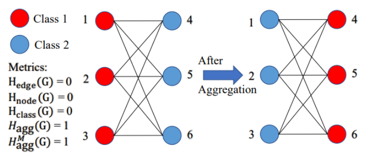
Figure \ref{Figure:4} shows that the majority of homophily metrics result in zeros, indicating heterophily. As a consequence, classes 1 and 2 cannot be distinguished based on these metrics. However, after mean aggregation, nodes in classes 1 and 2 merely swap colors and remain distinguishable. This example highlights the importance of examining the relationship between nodes following the aggregation step, in addition to ensuring graph-label consistency. To address this, this paper begin by defining the post-aggregation node similarity matrix as follows: \begin{equation} S(\hat{A},X) = \hat{A}X(\hat{A}X)^T \in \mathbb{R}^{N\times N} \end{equation}
where \(\hat{A} \in \mathbb{R}^{N \times N}\) denotes a general aggregation operator. \(S(\hat{A}, X)\) is the gram matrix that measures the similarity between each pair of aggregated node features.
Adaptive Channel Mixing (ACM)
In previous studies [13] [7] [14], it has been established that leveraging high-frequency graph signals, attainable through the application of a high-pass filter (HP), has proven to be empirically beneficial in handling heterophily.
Another concept presented in this paper is that, unlike the majority of existing GNNs that employ a single-channel filtering architecture [15] [16] [17] utilizing either a low-pass filter or a high-pass filter channel, which only partially retains the input information, the use of filterbanks with \(H_{LP} + H_{HP} = I\) ensures that no information is lost from the input signal (Adaptive Channel Mixing).
Geometric Knowledge Distillation: Topology Compression for Graph Neural Networks [18]
GNNs heavily depend on the structure and topology of the graph. This paper focuses on identifying the graph’s topology, referred to as ‘Geometric Knowledge’ in this context, from a thermodynamic perspective.
This paper revisits the connection between thermodynamics and the behavior of GNNs. Building on this connection, the paper introduces the concept of the Neural Heat Kernel (NHK) to capture the geometric characteristics of the underlying manifold with respect to GNN architecture.
Towards the end, a novel approach to knowledge transfer emerges, aiming to encode graph topological information into Graph Neural Networks (GNNs). This is achieved through knowledge distillation, where information is transferred from a teacher GNN model trained on a complete graph to a student GNN model operating on a smaller or sparser graph. This alignment of NHKs between teacher and student models is referred to as Geometric Knowledge Distillation.
Heat Kernel and Extending it to GNNs
The heat kernel represents the unique solution to the heat equation in thermodynamics, capturing the underlying structure of the equation. In simpler terms, it provides a distinct representation of the equation’s geometry. GNNs and the heat equation exhibit similarities, allowing us to extend the concept of the heat kernel to GNNs, referred to as the Neural Heat Kernel (NHK), to obtain the underlying representation of a graph.
This paper demonstrates that there is a unique NHK for each GNN. Once the NHK is obtained for a particular GNN, it can be employed as a function in each layer of the neural network.
\begin{equation} h_v^{(l)} = \sum_{u \in V} k^{(l)}(v,u).h_u^{(l-1)} \mu(u) \end{equation}
Where \(K\) is the (NHK) at layer \(l\), and \(\mu\) is the inverse of the nodee degree.
Geometric Knowledge Distillation (GKD)
The problem of distilling geometric knowledge involves an intelligent teacher model, which is trained on the complete graph \(\tilde{G}\), and a student model exposed to the partial graph \(G\). NHK matrices should be constructed for both models, and the loss function should utilize both of these matrices. Consequently, a Frobenius norm over these two matrices could be employed.
Deep Generative Model for Periodic Graphs [19]
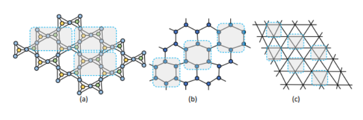
Creating periodic graphs presents several challenges, including 1) preserving graph periodicity, 2) distinguishing between local and global patterns, and 3) efficiently learning repetitive patterns. This paper introduces a novel deep generative model for periodic graphs that can autonomously acquire, separate, and generate both local and global graph patterns.
PGD-VAE architecture
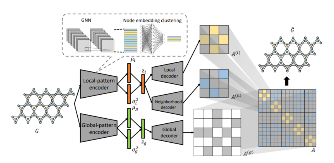
Figure 6 illustrates the proposed architecture in this paper. In this paper, the periodic sections of the graph are referred to as basic units, containing local information of the graph. First, there is an encoder for encoding the graph into the latent space. This encoder should be capable of learning close representations for graphs with the same basic units and distinct representations for other cases. As a result, two encoders are used: one for encoding local information and the other for encoding global information.
For the decoder, three decoders are utilized. One takes the latent representations of local information as input and is responsible for reconstructing these basic units. The third decoder performs the same task with the latent representation of global information, while the second decoder employs both representations to learn how to assemble basic units. Finally, the loss function consists of three components, with two parts resembling existing loss functions in VAEs. However, there is an additional part (part 3) that minimizes the Kullback–Leibler (KL) divergence between the true prior and the approximated posterior distributions to encourage the disentanglement of local and global representations.
[1] B. Weisfeiler and A. Leman, “The reduction of a graph to canonical form and the algebra which appears therein,” nti, Series, vol. 2, no. 9, pp. 12–16, 1968.
[2] W. L. Hamilton, Graph representation learning. Morgan & Claypool Publishers, 2020.
[3] P. W. Battaglia et al., “Relational inductive biases, deep learning, and graph networks,” arXiv preprint arXiv:1806.01261, 2018.
[4] J. Zhu, Y. Yan, L. Zhao, M. Heimann, L. Akoglu, and D. Koutra, “Beyond homophily in graph neural networks: Current limitations and effective designs,” Advances in neural information processing systems, vol. 33, pp. 7793–7804, 2020.
[5] M. Zhang and P. Li, “Nested graph neural networks,” Advances in Neural Information Processing Systems, vol. 34, pp. 15 734–15 747, 2021.
[6] J. Feng, Y. Chen, F. Li, A. Sarkar, and M. Zhang, “How powerful are k-hop message passing graph neural networks,” Advances in Neural Information Processing Systems, vol. 35, pp. 4776–4790, 2022.
[7] E. Chien, J. Peng, P. Li, and O. Milenkovic, “Adaptive universal generalized pagerank graph neural network,” arXiv preprint arXiv:2006.07988, 2020.
[8] S. Abu-El-Haija et al., “Mixhop: Higher-order graph convolutional architectures via spar- sified neighborhood mixing,” in international conference on machine learning, PMLR, 2019, pp. 21–29.
[9] R. Brossard, O. Frigo, and D. Dehaene, “Graph convolutions that can finally model local structure,” arXiv preprint arXiv:2011.15069, 2020.
[10] C. Ying et al., “Do transformers really perform badly for graph representation?” Advances in Neural Information Processing Systems, vol. 34, pp. 28 877–28 888, 2021.
[11] S. Luan et al., “Revisiting heterophily for graph neural networks,” Advances in neural information processing systems, vol. 35, pp. 1362–1375, 2022.
[12] M. McPherson, L. Smith-Lovin, and J. M. Cook, “Birds of a feather: Homophily in social networks,” Annual review of sociology, vol. 27, no. 1, pp. 415–444, 2001.
[13] S. Luan, M. Zhao, C. Hua, X.-W. Chang, and D. Precup, “Complete the missing half: Augmenting aggregation filtering with diversification for graph convolutional networks,” arXiv preprint arXiv:2008.08844, 2020.
[14] D. Bo, X. Wang, C. Shi, and H. Shen, “Beyond low-frequency information in graph convolutional networks,” in Proceedings of the AAAI Conference on Artificial Intelligence, vol. 35, 2021, pp. 3950–3957.
[15] T. N. Kipf and M. Welling, “Semi-supervised classification with graph convolutional networks,” arXiv preprint arXiv:1609.02907, 2016.
[16] P. Veličković, G. Cucurull, A. Casanova, A. Romero, P. Lio, and Y. Bengio, “Graph attention networks,” arXiv preprint arXiv:1710.10903, 2017.
[17] W. Hamilton, Z. Ying, and J. Leskovec, “Inductive representation learning on large graphs,” Advances in neural information processing systems, vol. 30, 2017.
[18] C. Yang, Q. Wu, and J. Yan, “Geometric knowledge distillation: Topology compression for graph neural networks,” Advances in Neural Information Processing Systems, vol. 35, pp. 29 761–29 775, 2022.
[19] S. Wang, X. Guo, and L. Zhao, “Deep generative model for periodic graphs,” Advances in Neural Information Processing Systems, vol. 35, 2022.
The pdf of the report is also available: